nlcpy.fft.fft

nlcpy.fft.fft(a, n=None, axis=- 1, norm=None)[ソース]

Computes the one-dimensional discrete fourier transform.

This function computes the one-dimensional n-point discrete fourier transform (DFT) with the efficient fast fourier transform (FFT) algorithm.

Parameters

aarray_like: Input array, can be complex.
nint,optional: Length of the transformed axis of the output. If n is smaller than the length of the input, the input is cropped. If it is larger, the input is padded with zeros. If n is not given, the length of the input along the axis specified by axis is used.
axisint,optional: Axis over which to compute the FFT. If not given, the last axis is used. If axis is larger than the last axis of a, IndexError occurs.
norm{None, "ortho"},optional: Normalization mode. By default(None), the transforms are unscaled. It norm is set to "ortho", the return values will be scaled by $1/\sqrt{n}$ .

Returns

outcomplex ndarray: The truncated or zero-padded input, transformed along the axis indicated by axis , or the last one if axis is not specified.

参考

ifft: Computes the one-dimensional inverse discrete fourier transform.
fft2: Computes the 2-dimensional discrete fourier transform.
fftn: Computes the n-dimensional discrete fourier transform.
rfftn: Computes the n-dimensional discrete fourier transform for a real array.
fftfreq: Returns the discrete fourier transform sample frequencies.

注釈

FFT (fast fourier transform) refers to a way the discrete fourier transform (DFT) can be calculated efficiently, by using symmetries in the calculated terms. The symmetry is highest when n is a power of 2, and the transform is therefore most efficient for these sizes.

Examples

>>> import nlcpy as vp
>>> vp.fft.fft(vp.exp(2j * vp.pi * vp.arange(8) / 8))    
array([-3.44509285e-16+1.14423775e-17j,  8.00000000e+00-8.52069395e-16j,
        2.33486982e-16+1.22464680e-16j,  0.00000000e+00+1.22464680e-16j,
        9.95799250e-17+2.33486982e-16j,  0.00000000e+00+1.17281316e-16j,
        1.14423775e-17+1.22464680e-16j,  0.00000000e+00+1.22464680e-16j])

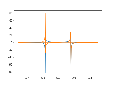
In this example, real input has an FFT which is Hermitian, i.e., symmetric in the real part and anti-symmetric in the imaginary part:

>>> import matplotlib.pyplot as plt
>>> t = vp.arange(256)
>>> sp = vp.fft.fft(vp.sin(t))
>>> freq = vp.fft.fftfreq(t.shape[-1])
>>> _ = plt.plot(freq, sp.real, freq, sp.imag)
>>> plt.show()