nlcpy.fft.fftn

nlcpy.fft.fftn(a, s=None, axes=None, norm=None)[ソース]

Computes the n-dimensional discrete fourier transform.

This function computes the n-dimensional discrete fourier transform over any number of axes in an m-dimensional array by means of the fast fourier transform (FFT).

Parameters

aarray_like: Input array, can be complex.
ssequence of ints, optional: Shape (length of each transformed axis) of the output (s[0] refers to axis 0, s[1] to axis 1, etc.). This corresponds to n for fft(x, n). Along any axis, if the given shape is smaller than that of the input, the input is cropped. If it is larger, the input is padded with zeros. if s is not given, the shape of the input along the axes specified by axes is used. If s and axes have different length, ValueError occurs.
axessequence of ints, optional: Axes over which to compute the FFT. If not given, the last len(s) axes are used, or all axes if s is also not specified. Repeated indices in axes means that the transform over that axis is performed multiple times. If an element of axes is larger than than the number of axes of a, IndexError occurs.
norm{None, "ortho"},optional: Normalization mode. By default(None), the transforms are unscaled. It norm is set to "ortho", the return values will be scaled by $1/\sqrt{n}$ .

Returns

outcomplex ndarray: The truncated or zero-padded input, transformed along the axes indicated by axes, or by a combination of s and a, as explained in the parameters section above.

参考

ifftn: Computes the n-dimensional inverse discrete fourier transform.
fft: Computes the one-dimensional discrete fourier transform.
rfftn: Computes the n-dimensional discrete fourier transform for a real array.
fft2: Computes the 2-dimensional discrete fourier transform.
fftshift: Shifts the zero-frequency component to the center of the spectrum.

注釈

The output, analogously to fft(), contains the term for zero frequency in the low-order corner of all axes, the positive frequency terms in the first half of all axes, the term for the Nyquist frequency in the middle of all axes and the negative frequency terms in the second half of all axes, in order of decreasingly negative frequency.

Examples

>>> import nlcpy as vp
>>> import numpy as np
>>> a = np.mgrid[:3, :3, :3][0]
>>> vp.fft.fftn(a, axes=(1, 2))
array([[[ 0.+0.j,  0.+0.j,  0.+0.j],
        [ 0.+0.j,  0.+0.j,  0.+0.j],
        [ 0.+0.j,  0.+0.j,  0.+0.j]],

       [[ 9.+0.j,  0.+0.j,  0.+0.j],
        [ 0.+0.j,  0.+0.j,  0.+0.j],
        [ 0.+0.j,  0.+0.j,  0.+0.j]],

       [[18.+0.j,  0.+0.j,  0.+0.j],
        [ 0.+0.j,  0.+0.j,  0.+0.j],
        [ 0.+0.j,  0.+0.j,  0.+0.j]]])
>>> vp.fft.fftn(a, (2, 2), axes=(0, 1))
array([[[ 2.+0.j,  2.+0.j,  2.+0.j],
        [ 0.+0.j,  0.+0.j,  0.+0.j]],

       [[-2.+0.j, -2.+0.j, -2.+0.j],
        [ 0.+0.j,  0.+0.j,  0.+0.j]]])

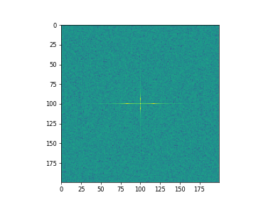
>>> import matplotlib.pyplot as plt
>>> [X, Y] = np.meshgrid(2 * vp.pi * vp.arange(200) / 12,
...                      2 * vp.pi * vp.arange(200) / 34)
>>> S = vp.sin(X) + vp.cos(Y) + vp.random.uniform(0, 1, X.shape)
>>> FS = vp.fft.fftn(S)
>>> _ = plt.imshow(vp.log(vp.absolute(vp.fft.fftshift(FS))**2))
>>> plt.show()